It’s well known that the GOR of oil wells can change over time, usually increasing, so it’s important to have the flexibility to model that. Our decline curves have the ability to model multiple segments of GOR changes over time. Rather than modeling gas in an independent stream, engineers can create model forecasts using GOR. This workflow shows you how to apply a GOR using the Forecast Scenarios App.
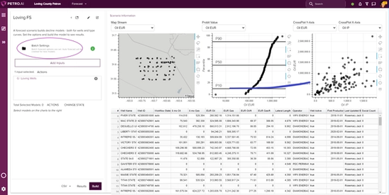
After the decline curve is generated in a Forecast Scenario, click on Batch Settings.
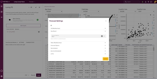
In the Forecast Settings popup, set Gas from Modified Arps to None so a gas curve isn’t fitted. Click Update.
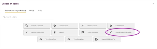
Select the well you’d like to analyze from the summary table. It’s added to Total Selected Models. Click on ACTIONS.
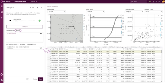
In the Choose an action popup, click on Edit the Decline Curve Model.
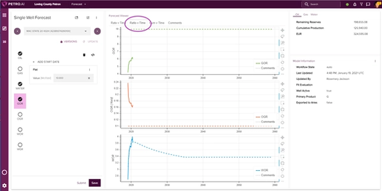
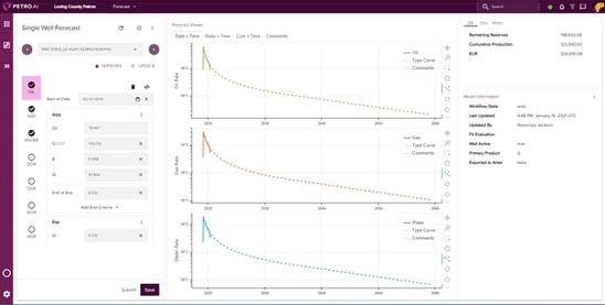
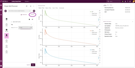
This takes you to the Single Well Forecast page that has the production history, the forecast that was fit and all the parameters.
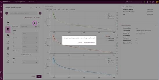
Once the curves have been generated through the autofit, you can remove a curve by clicking on GAS on the right panel and then the trash icon. Click on REMOVE SEGMENTS from gas in the popup.
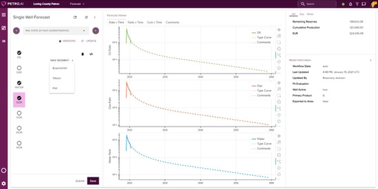
Click on GOR on the right panel, now highlighted in pink and click ADD SEGMENTS. NEW SEGMENT pops up. Click the dropdown and select Exponential, Values or Flat. Values change over time and flat stays constant. Once changed, click Update.
Here we’ve chosen flat and changed the Mcf/bbls to 10. Click Update.
In the Forecast Viewer, click on the Ratio v Time tab to see the ratio plots including GOR.